So, yeah, the use of “hacks” in the title is definitely on the ironic and gratuitous side, but there is still a point to be made: are you making full use of current technology to keep your tests secure?  Gone are the days when you are limited to linear test forms on paper in physical locations.  Here are some quick points on how modern assessment technology can deliver assessments more securely, effectively, and efficiently than traditional methods:

1.  AI delivery like CAT and LOFT

Psychometrics was one of the first areas to apply modern data science and machine learning (see this blog post for a story about a MOOC course).  But did you know it was also one of the first areas to apply artificial intelligence (AI)?  Early forms of computerized adaptive testing (CAT) were suggested in the 1960s and had become widely available in the 1980s.  CAT delivers a unique test to each examinee by using complex algorithms to personalize the test.  This makes it much more secure, and can also reduce test length by 50-90%.

2. Psychometric forensics

Modern psychometrics has suggested many methods for finding cheaters and other invalid test-taking behavior.  These can range from very simple rules like flagging someone for having a top 5% score in a bottom 5% time, to extremely complex collusion indices.  These approaches are designed explicitly to keep your test more secure.

3. Tech enhanced items

Tech enhanced items (TEIs) are test questions that leverage technology to be more complex than is possible on paper tests.  Classic examples include drag and drop or hotspot items.  These items are harder to memorize and therefore contribute to security.

4. IP address limits

Suppose you want to make sure that your test is only delivered in certain school buildings, campuses, or other geographic locations.  You can build a test delivery platform that limits your tests to a range of IP addresses, which implements this geographic restriction.

5. Lockdown browser

A lockdown browser is a special software that locks a computer screen onto a test in progress, so for example a student cannot open Google in another tab and simply search for answers.  Advanced versions can also scan the computer for software that is considered a threat, like a screen capture software.

6. Identity verification

Tests can be built to require unique login procedures, such as requiring a proctor to enter their employee ID and the test-taker to enter their student ID.  Examinees can also be required to show photo ID, and of course, there are new biometric methods being developed.

7. Remote proctoring

The days are gone when you need to hop in the car and drive 3 hours to sit in a windowless room at a community college to take a test.  Nowadays, proctors can watch you and your desktop via webcam.  This is arguably as secure as in-person proctoring, and certainly more convenient and cost-effective.

So, how can I implement these to deliver assessments more securely?

Some of these approaches are provided by vendors specifically dedicated to that space, such as ProctorExam for remote proctoring.  However, if you use ASC’s FastTest platform, all of these methods are available for you right out of the box.  Want to see for yourself?  Sign up for a free account!

The traditional Learning Management System (LMS) is designed to serve as a portal between educators and their learners. Platforms like Moodle are successful in facilitating cooperative online learning in a number of groundbreaking ways: course management, interactive discussion boards, assignment submissions, and delivery of learning content. While all of this is great, we’ve yet to see an LMS that implements best practices in assessment and psychometrics to ensure that medium or high stakes tests meet international standards.

To put it bluntly, LMS systems have assessment functionality that is usually good enough for short classroom quizzes but falls far short of what is required for a test that is used to award a credential.  A white paper on this topic is available here, but some examples include:

  • Treatment of items as reusable objects
  • Item metadata and historical use
  • Collaborative item review and versioning
  • Test assembly based on psychometrics
  • Psychometric forensics to search for non-independent test-taking behavior
  • Deeper score reporting and analytics

Assessment Systems is pleased to announce the launch of an easy-to-use bridge between FastTest and Moodle that will allow users to seamlessly deliver sound assessments from within Moodle while taking advantage of the sophisticated test development and psychometric tools available within FastTest. In addition to seamless delivery for learners, all candidate information is transferred to FastTest, eliminating the examinee import process.  The bridge makes use of the international Learning Tools Interoperability standards.

If you are already a FastTest user, watch a step-by-step tutorial on how to establish the connection, in the FastTest User Manual by logging into your FastTest workspace and selecting Manual in the upper right-hand corner. You’ll find the guide in Appendix N.

If you are not yet a FastTest user and would like to discuss how it can improve your assessments while still allowing you to leverage Moodle or other LMS systems for learning content, sign up for a free account here.

One of my graduate school mentors once said in class that there are three standard errors that everyone in the assessment or I/O Psych field needs to know: mean, error, and estimate.  They are quite distinct in concept and application but easily confused by someone with minimal training.

I’ve personally seen the standard error of the mean reported as the standard error of measurement, which is completely unacceptable.

So in this post, I’ll briefly describe each so that the differences are clear.  In later posts, I’ll delve deeper into each of the standard errors.


Standard Error of the Mean

This is the standard error that you learned about in Introduction to Statistics back in your sophomore year of college/university.  It is related to the Central Limit Theorem, the cornerstone of statistics.  Its purpose is to provide an index of accuracy (or conversely, error) in a sample mean.  Any sample drawn from a population will have an average, but these can vary.  The standard error of the mean estimates the variation we might expect in these different means from different samples and is defined as

   SEmean = SD/sqrt(n)

Where SD is the sample’s standard deviation and n is the number of observations in the sample.  This can be used to create a confidence interval for the true population mean.

The most important thing to note, with respect to psychometrics, is that this has nothing to do with psychometrics.  This is just general statistics.  You could be weighing a bunch of hay bales and calculating their average; anything where you are making observations.  It can be used, however, with assessment data.

For example, if you do not want to make every student in a country take a test, and instead sample 50,000 students, with a mean of 71 items correct with an SD of 12.3, then the SEM is  12.3/sqrt(50000) = 0.055.  You can be 95% certain that the true population means then lies in the narrow range of 71 +- 0.055.

Click here to read more.

Standard Error of Measurement

More important in the world of assessment is the standard error of measurement.  Its purpose is to provide an index of the accuracy of a person’s score on a test.  That is a single person, rather than a group like with the standard error of the mean.  It can be used in both the classical test theory perspective and item response theory perspective, though it is defined quite differently in both.

In classical test theory, it is defined as

   SEM = SD*sqrt(1-r)

Where SD is the standard deviation of scores for everyone who took the test, and r is the reliability of the test.  It can be interpreted as the standard deviation of scores that you would find if you had the person take the test over and over, with a fresh mind each time.  A confidence interval with this is then interpreted as the band where you would expect the person’s true score on the test to fall.

Item Response Theory conceptualizes the SEM as a continuous function across the range of student abilities.  A test form will have more accuracy – less error – in a range of abilities where there are more items or items of higher quality.  That is, a test with most items of middle difficulty will produce accurate scores in the middle of the range, but not measure students on the top or bottom very well.  The example below is a test that has many items above the average examinee score (θ) of 0.0 so that any examinee with a score of less than 0.0 has a relatively inaccurate score, namely with an SEM greater than 0.50.


Standard error of measurement and test information function

For a deeper discussion of SEM, click here.


Standard Error of the Estimate

Lastly, we have the standard error of the estimate.  This is an estimate of the accuracy of a prediction that is made, usually in the paradigm of linear regression.  Suppose we are using scores on a 40 item job knowledge test to predict job performance, and we have data on a sample of 1,000 job incumbents that took the test last year and have job performance ratings from this year on a measure that entails 20 items scored on a 5 point scale for a total of 100 points.

There might have been 86 incumbents that scored 30/40 on the test, and they will have a range of job performance, let’s say from 61 to 89.  If a new person takes the test and scores 30/40, how would we predict their job performance?

The SEE is defined as

       SEE = SDy*sqrt(1-r2)

Here, the r is the correlation of x and y, not reliability. Many statistical packages can estimate linear regression, SEE, and many other related statistics for you.  In fact, Microsoft Excel comes with a free package to implement simple linear regression.  Excel estimates the SEE as 4.69 in the example above, and the regression slope and intercept are 29.93 and 1.76, respectively

Given this, we can estimate the job performance of a person with a 30 test score to be 82.73.  A 95% confidence interval for a candidate with a test score of 30 is then 82.71-(4.69*1.96) to 82.71+(4.69*1.96), or 73.52 to 91.90.

You can see how this might be useful in prediction situations.  Suppose we wanted to be sure that we only hired people who are likely to have a job performance rating of 80 or better?  Well, a cutscore of 30 on the test is therefore quite feasible.


OK, so now what?

Well, remember that these three standard errors are quite different and are not even in related situations.  When you see a standard error requested – for example if you must report the standard error for an assessment – make sure you use the right one!

Validity, in its modern conceptualization, refers to evidence that supports our intended interpretations of test scores (see Chapter 1 of APA/AERA/NCME Standards for full treatment).  Validity threats are issues that hinder the interpretations and use of scores.  The word “interpretation” is key because test scores can be interpreted in different ways, including ways that are not intended by the test designers.

For example, a test given at the end of Nursing school to prepare for a national licensure exam might be used by the school as a sort of Final Exam.  However, the test was not designed for this purpose and might not even be aligned with the school’s curriculum.

Another example is that certification tests are usually designed to demonstrate minimal competence, not differentiate amongst experts, so interpreting a high score as expertise might not be warranted.

Validity threats: Always be on the lookout!

Test sponsors, therefore, must be vigilant against any validity threats.  Some of these, like the two aforementioned examples, might be outside the scope of the organization.  While it is certainly worthwhile to address such issues, our primary focus is on aspects of the exam itself.

Which validity threats rise to the surface in psychometric forensics?

Here, we will discuss several threats to validity that typically present themselves in psychometric forensics, with a focus on security aspects.  However, I’m not just listing security threats here, as psychometric forensics is excellent at flagging other types of validity threats too.

Threat Description Approach Example Indices
Collusion (copying) Examinees are copying answers from one another, usually with a defined Source. Error similarity (only looks at incorrect) 2 examinees get the same 10 items wrong, and select the same distractor on each B-B Ran, B-B Obs, K, K1, K2, S2
Response similarity 2 examinees give the same response on 98/100 items S2, g2, ω, Zjk
Group level help/issues Similar to collusion but at a group level; could be examinees working together, or receiving answers from a teacher/proctor.  Note that many examinees using the same brain dump would have a similar signature but across locations. Group level statistics Location has one of the highest mean scores but lowest mean times Descriptive statistics such as mean score, mean time, and pass rate
Response or error similarity On a certain group of items, the entire classroom gives the same answers Roll-up analysis, such as mean collusion flags per group; also erasure analysis (paper only)
Pre-Knowledge Examinee comes in to take the test already knowing the items and answers, often purchased from a brain dump website. Time-Score analysis Examinee has high score and very short time RTE or total time vs. scores
Response or error similarity Examinee has all the same responses as a known brain dump site All indices
Pretest item comparison Examinee gets 100% on existing items but 50% on new items Pre vs Scored results
Person fit Examinee gets the 10 hardest items correct but performs below average on the rest of the items Guttman indices, lz
Harvesting Examinee is not actually taking the test, but is sitting it to memorize items so they can be sold afterwards, often at a brain dump website.  Similar signature to Sleepers but more likely to occur on voluntary tests, or where high scores benefit examinees. Time-Score analysis Low score, high time, few attempts. RTE or total time vs. scores
Mean vs Median item time Examinee “camps” on 10 items to memorize them; mean item time much higher than the median Mean-Median index
Option flagging Examinee answers “C” to all items in the second half Option proportions
Low motivation: Sleeper Examinees are disengaged, producing data that is flagged as unusual and invalid; fortunately, not usually a security concern but could be a policy concern. Similar signature to Harvester but more likely to occur on mandatory tests, or where high scores do not benefit examinees. Time-Score analysis Low score, high time, few attempts. RTE or total time vs. scores
Item timeout rate If you have item time limits, examinee hits them Proportion items that hit limit
Person fit Examinee attempt a few items, passes through the rest Guttman indices, lz
Low motivation: Clicker Examinees are disengaged, producing data that is flagged as unusual and invalid; fortunately, not usually a security concern but could be a policy concern. Similar idea to Sleeper but data is quite different. Time-Score analysis Examinee quickly clicks “A” to all items, finishing with a low time and low score RTE, Total time vs. scores
Option flagging See above Option proportions

One of the core concepts in psychometrics is item difficulty.  This refers to the probability that examinees will get the item correct for educational/cognitive assessments or respond in the keyed direction with psychological/survey assessments (more on that later).  Difficulty is important for evaluating the characteristics of an item and whether it should continue to be part of the assessment; in many cases, items are deleted if they are too easy or too hard.  It also allows us to better understand how the items and test as a whole operate as a measurement instrument, and what they can tell us about examinees.

I’ve heard of “item facility.” Is that similar?

Item difficulty is also called item facility, which is actually a more appropriate name.  Why?  The P value is a reverse of the concept: a low value indicates high difficulty, and vice versa.  If we think of the concept as facility or easiness, then the P value aligns with the concept; a high value means high easiness.  Of course, it’s hard to break with tradition, and almost everyone still calls it difficulty.  But it might help you here to think of it as “easiness.”

How do we calculate classical item difficulty?

There are two predominant paradigms in psychometrics: classical test theory (CTT) and item response theory (IRT).  Here, I will just focus on the simpler approach, CTT.

To calculate classical item difficulty with dichotomous items, you simply count the number of examinees that responded correctly (or in the keyed direction) and divide by the number of respondents.  This gets you a proportion, which is like a percentage but is on the scale of 0 to 1 rather than 0 to 100.  Therefore, the possible range that you will see reported is 0 to 1.  Consider this data set.

Person Item1 Item2 Item3 Item4 Item5 Item6 Score
1 0 0 0 0 0 1 1
2 0 0 0 0 1 1 2
3 0 0 0 1 1 1 3
4 0 0 1 1 1 1 4
5 0 1 1 1 1 1 5
Diff: 0.00 0.20 0.40 0.60 0.80 1.00

Item6 has a high difficulty index, meaning that it is very easy.  Item4 and Item5 are typical items, where the majority of items are responding correctly.  Item1 is extremely difficult; no one got it right!

For polytomous items (items with more than one point), classical item difficulty is the mean response value.  That is, if we have a 5 point Likert item, and two people respond 4 and two response 5, then the average is 4.5.  This, of course, is mathematically equivalent to the P value if the points are 0 and 1 for a no/yes item.  An example of this situation is this data set:

Person Item1 Item2 Item3 Item4 Item5 Item6 Score
1 1 1 2 3 4 5 1
2 1 2 2 4 4 5 2
3 1 2 3 4 4 5 3
4 1 2 3 4 4 5 4
5 1 2 3 5 4 5 5
Diff: 1.00 1.80 2.60 4.00 4.00 5.00

Note that this is approach to calculating difficulty is sample-dependent.  If we had a different sample of people, the statistics could be quite different.  This is one of the primary drawbacks to classical test theory.  Item response theory tackles that issue with a different paradigm.  It also has an index with the right “direction” – high values mean high difficulty with IRT.

If you are working with multiple choice items, remember that while you might have 4 or 5 responses, you are still scoring the items as right/wrong.  Therefore, the data ends up being dichotomous 0/1.

Very important final note: this P value is NOT to be confused with p value from the world of hypothesis testing.  They have the same name, but otherwise are completely unrelated.  For this reason, some psychometricians call it P+ (pronounced “P-plus”), but that hasn’t caught on.

How do I interpret classical item difficulty?

For educational/cognitive assessments, difficulty refers to the probability that examinees will get the item correct.  If more examinees get the item correct, it has low difficulty.  For psychological/survey type data, difficulty refers to the probability of responding in the keyed direction.  That is, if you are assessing Extraversion, and the item is “I like to go to parties” then you are evaluating how many examinees agreed with the statement.

What is unique with survey type data is that it often includes reverse-keying; the same assessment might also have an item that is “I prefer to spend time with books rather than people” and an examinee disagreeing with that statement counts as a point towards the total score.

For the stereotypical educational/knowledge assessment, with 4 or 5 option multiple choice items, we use general guidelines like this for interpretation.

Range Interpretation Notes
0.0-0.3 Extremely difficult Examinees are at chance level or even below, so your item might be miskeyed or have other issues
0.3-0.5 Very difficult Items in this range will challenge even top examinees, and therefore might elicit complaints, but are typically very strong
0.5-0.7 Moderately difficult These items are fairly common, and a little on the tougher side
0.7-0.90 Moderately easy These are the most common range of items on most classically built tests; easy enough that examinees rarely complain
0.90-1.0 Very easy These items are mastered by most examinees; they are actually too easy to provide much info on examinees though, and can be detrimental to reliability.

Do I need to calculate this all myself?

No.  There is plenty of software to do it for you.  If you are new to psychometrics, I recommend CITAS, which is designed to get you up and running quickly but is too simple for advanced situations.  If you have large samples or are involved with production-level work, you need Iteman.  Sign up for a free account with the button below.  If that is you, I also recommend that you look into learning IRT if you have not yet.

Item banking refers to the purposeful creation of a database of assessment items to serve as a central repository of all test content, improving efficiency and quality. The term item refers to what many call questions; though their content need not be restricted as such and can include problems to solve or situations to evaluate in addition to straightforward questions. As a critical foundation to the test development cycle, item banking is the foundation for the development of valid, reliable content and defensible test forms.

Automated item banking systems, such as Assess.ai or FastTest, result in significantly reduced administrative time for developing/reviewing items and assembling/publishing tests, while producing exams that have greater reliability and validity.  Contact us to request a free account.


What is Item Banking?

While there are no absolute standards in creating and managing item banks, best practice guidelines are emerging. Here are the essentials your should be looking for:

   Items are reusable objects; when selecting an item banking platform it is important to ensure that items can be used more than once; ideally, item performance should be tracked not only within a test form but across test forms as well.

   Item history and usage are tracked; the usage of a given item, whether it is actively on a test form or dormant waiting to be assigned, should be easily accessible for test developers to assess, as the over-exposure of items can reduce the validity of a test form. As you deliver your items, their content is exposed to examinees. Upon exposure to many examinees, items can then be flagged for retirement or revision to reduce cheating or teaching to the test.

   Items can be sorted; as test developers select items for a test form, it is imperative that they can sort items based on their content area or other categorization methods, so as to select a sample of items that is representative of the full breadth of constructs we intend to measure.

   Item versions are tracked; as items appear on test forms, their content may be revised for clarity. Any such changes should be tracked and versions of the same item should have some link between them so that we can easily review the performance of earlier versions in conjunction with current versions.

   Review process workflow is tracked; as items are revised and versioned, it is imperative that the changes in content and the users who made these changes are tracked. In post-test assessment, there may be a need for further clarification, and the ability to pinpoint who took part in reviewing an item and expedite that process.

   Metadata is recorded; any relevant information about an item should be recorded and stored with the item. The most common applications for metadata that we see are author, source, description, content area, depth of knowledge, IRT parameters, and CTT statistics, but there are likely many data points specific to your organization that is worth storing.

Managing an Item Bank

Names are important. As you create or import your item banks it is important to identify each item with a unique, but recognizable name. Naming conventions should reflect your bank’s structure and should include numbers with leading zeros to support true numerical sorting.  You might want to also add additional pieces of information.  If importing, the system should be smart enough to recognize duplicates.

Search and filter. The system should also have a reliable sorting mechanism. 

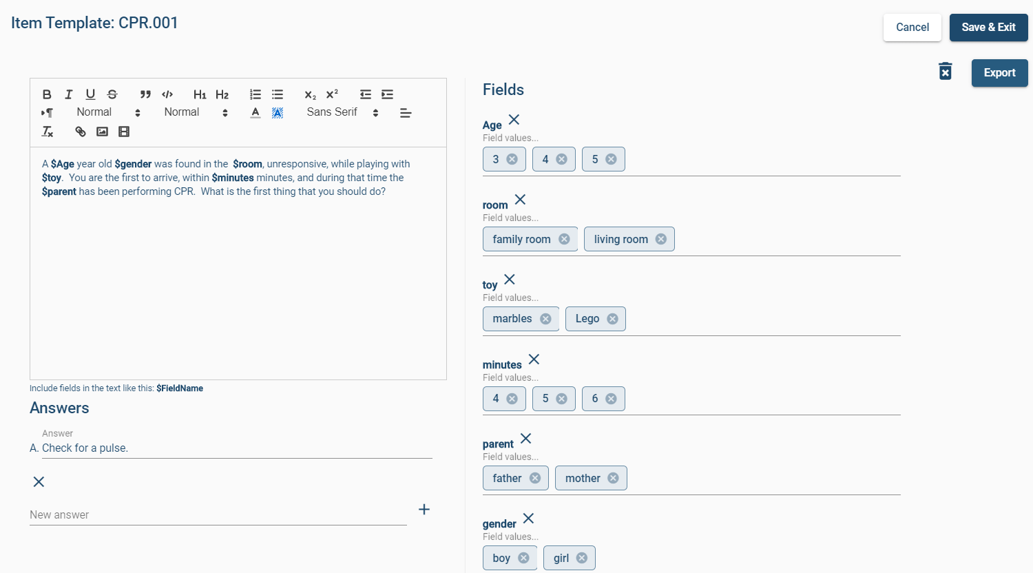
automated item generation cpr

Prepare for the Future: Store Extensive Metadata

Metadata is valuable. As you create items, take the time to record simple metadata like author and source. Having this information can prove very useful once the original item writer has moved to another department, or left the organization. Later in your test development life cycle, as you deliver items, you have the ability to aggregate and record item statistics. Values like discrimination and difficulty are fundamental to creating better tests, driving reliability, and validity.

Statistics are used in the assembly of test forms while classical statistics can be used to estimate mean, standard deviation, reliability, standard error, and pass rate. 

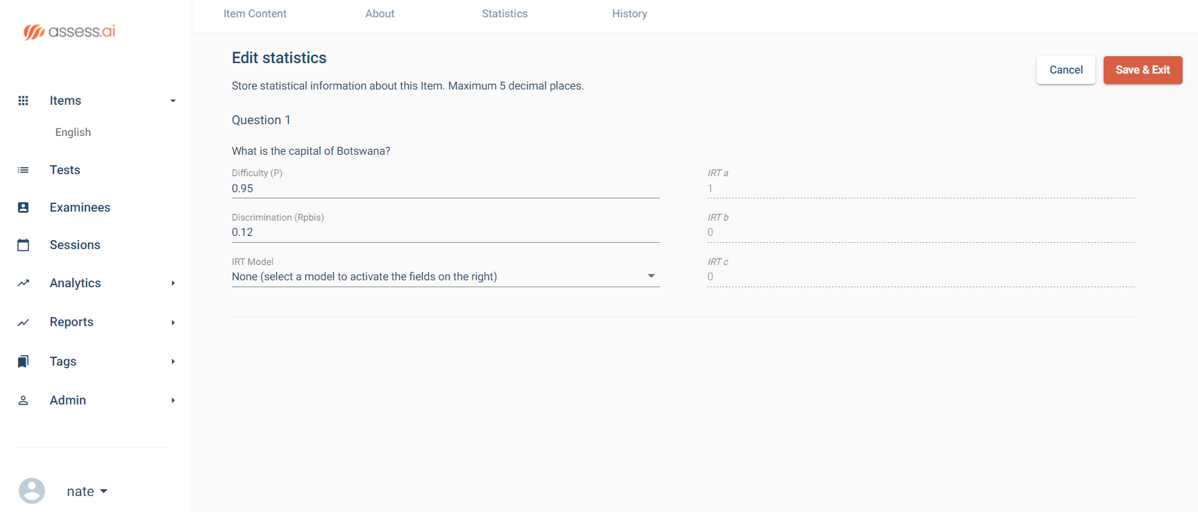
Item banking statistics

Item response theory parameters can come in handy when calculating test information and standard error functions. Data from both psychometric theories can be used to pre-equate multiple forms.

In the event that your organization decides to publish an adaptive test, utilizing CAT delivery, item parameters for each item will be essential. This is because they are used for intelligent selection of items and scoring examinees. Additionally, in the event that the integrity of your test or scoring mechanism is ever challenged, documentation of validity is essential to defensibility and the storage of metadata is one such vital piece of documentation.

Increase Content Quality: Track Workflow

Utilize a review workflow to increase quality. Using a standardized review process will ensure that all items are vetted in a similar matter. Have a step in the process for grammar, spelling, and syntax review, as well as content review by a subject matter expert. As an item progresses through the workflow, its development should be tracked, as workflow results also serve as validity documentation.

Accept comments and suggestions from a variety of sources. It is not uncommon for each item reviewer to view an item through their distinctive lens. Having a diverse group of item reviewers stands to benefit your test-takers, as they are likely to be diverse as well!

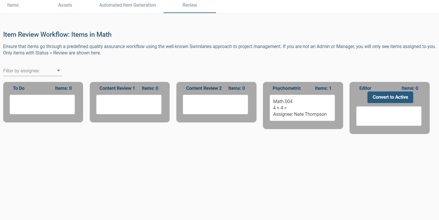
item review kanban

Keep Your Items Organized: Categorize Them

Identify items by content area. Creating a content hierarchy can also help you to organize your item bank and ensure that your test covers the relevant topics. Most often, we see content areas defined first by an analysis of the construct(s) being tested. In the event of a high school science test, this may include the evaluation of the content taught in class. A high-stakes certification exam, almost always includes a job-task analysis. Both methods produce what is called a test blueprint, indicating how important various content areas are to the demonstration of knowledge in the areas being assessed.

Once content areas are defined, we can assign items to levels or categories based on their content. As you are developing your test, and invariably referring back to your test blueprint, you can use this categorization to determine which items from each content area to select.

Why Item Banking?

There is no doubt that item banking is a key aspect of developing and maintaining quality assessments. Utilizing best practices, and caring for your items throughout the test development life cycle, will pay great dividends as it increases the reliability, validity, and defensibility of your assessment. Moreover, good item banking will make the job easier and more efficient thus reducing the cost of item development and test publishing.

Ready to improve assessment quality through item banking?

Visit our Contact Us page, where you can request a demonstration or a free account (up to 500 items).

A modified-Angoff method study is one of the most common ways to set a defensible cutscore on an exam.  If you have a criterion-referenced interpretation, it is not legally defensible to just conveniently pick a round number like 70%; you need a formal process.

There are a number of acceptable methodologies in the psychometric literature for standard-setting studies, also known as cutscores or passing points.  Some examples include Angoff, modified-Angoff, Bookmark, Contrasting Groups, and Borderline.The modified-Angoff approach is by far the popular approach. But, it remains a black box to many professionals in the testing industry, especially non-psychometricians in the credentialing field.  This post provides some clarity on the methodology. There is some flexibility in the study implementation, but this article describes a sound method.


What to Expect with the Modified-Angoff Method

First of all, do not expect a straightforward, easy process that leads to an unassailably correct cutscore.  All standard-setting methods involve some degree of subjectivity.  The goal of the methods is to reduce that subjectivity as much as possible.  Some methods focus on content, others on examinee performance data, while some try to meld the two.

Step 1: Prepare Your Team

The modified-Angoff process depends on a representative sample of subject matter experts (SMEs), usually 6-20.  By “representative” I mean they should represent the various stakeholders. For instance, a certification for medical assistants might include experienced medical assistants, nurses, and physicians, from different areas of the country.  You must train them about their role and how the process works, so they can understand the end goal and drive toward it.

Step 2: The Minimally Competent Candidate (MCC)

This concept is the core of the modified-Angoff method, though it is known by a range of terms or acronyms, including minimally qualified candidates (MQC) or just barely qualified (JBQ).  The reasoning is that we want our exam to separate candidates that are qualified from those that are not.  So we ask the SMEs to define what makes someone qualified (or unqualified!) from a perspective of skills and knowledge. This leads to a conceptual definition of an MCC.  We then want to estimate what score this borderline candidate would achieve, which is the goal of the remainder of the study.   This step can be conducted in person, or via webinar.

Step 3: Round 1 Ratings

Next, ask your SMEs to read through all the items on your test form and estimate the percentage of MCCs that would answer each correctly.  A rating of 100 means the item is a slam dunk; it is so easy that every MCC would get it right.  A rating of 40 is very difficult.  Most ratings are in the 60-90 range if the items are well-developed. The ratings should be gathered independently; if everyone is in the same room, let them work on their own in silence.  This can easily be conducted remotely, though.

Step 4: Discussion

This is where it gets fun.  Identify items where there is the most disagreement (as defined by grouped frequency distributions or standard deviation) and make the SMEs discuss it.  Maybe two SMEs thought it was super easy and gave it a 95 and two other SMEs thought it was super hard and gave it a 45.  They will try to convince the other side of their folly. Chances are that there will be no shortage of opinions and you, as the facilitator, will find your greatest challenge is keeping the meeting on track.  This step can be conducted in person, or via webinar.

Step 5: Round 2 Ratings

Raters then re-rate the items based on the discussion.  The goal is that there will be a greater consensus.  In the previous example, it’s not likely that every rater will settle on a 70.  But if your raters all end up from 60-80, that’s OK.  How do you know there is enough consensus?  We recommend the inter-rater reliability suggested by Shrout and Fleiss (1979), as well as looking at inter-rater agreement and dispersion of ratings for each item.  This use of multiple rounds is known as the Delphi approach; it pertains to all consensus-driven discussions in any field, not just psychometrics.

Step 6: Evaluate Results and Final Recommendation

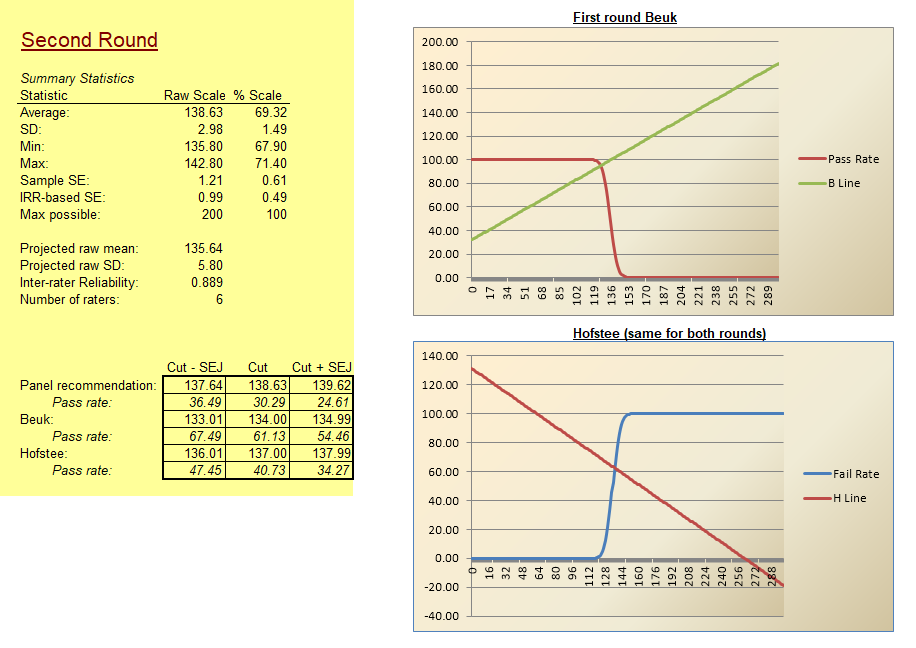
Evaluate the results from Round 2 as well as Round 1.  An example of this is below.  What is the recommended cutscore, which is the average or sum of the Angoff ratings depending on the scale you prefer?  Did the reliability improve?  Estimate the mean and SD of examinee scores (there are several methods for this). What sort of pass rate do you expect?  Even better, utilize the Beuk Compromise as a “reality check” between the modified-Angoff approach and actual test data.  You should take multiple points of view into account, and the SMEs need to vote on a final recommendation. They, of course, know the material and the candidates so they have the final say.  This means that standard setting is a political process; again, reduce that effect as much as you can.

Some organizations do not set the cutscore at the recommended point, but at one standard error of judgment (SEJ) below the recommended point.  The SEJ is based on the inter-rater reliability; note that it is NOT the standard error of the mean or the standard error of measurement.  Some organizations use the latter; the former is just plain wrong (though I have seen it used by amateurs).


modified angoff

Step 7: Write Up Your Report

Validity refers to evidence gathered to support test score interpretations.  Well, you have lots of relevant evidence here.  Document it.  If your test gets challenged, you’ll have all this in place.  On the other hand, if you just picked 70% as your cutscore because it was a nice round number, you could be in trouble.

Additional Topics

In some situations, there are more issues to worry about.  Multiple forms?  You’ll need to equate in some way.  Using item response theory?  You’ll have to convert the cutscore from the modified-Angoff method onto the theta metric using the Test Response Function (TRF).  New credential and no data available?  That’s a real chicken-and-egg problem there.

Where Do I Go From Here?

Ready to take the next step and actually apply the modified-Angoff process to improving your exams?   Sign up for a free account in our  FastTest item banker.

References

Shrout & Fleiss (1979). Intraclass correlations: Uses in assessing reliability. Psychological Bulletin, 86(2), 420-428.

I often hear this question about scaling, especially regarding the scaled scoring functionality found in software like FastTest and Xcalibre.  The following is adapted from lecture notes I wrote while teaching a course in Measurement and Assessment at the University of Cincinnati.

Test Scaling: Sort of a Tale of Two Cities

Scaling at the test level really has two meanings in psychometrics. First, it involves defining the method to operationally scoring the test, establishing an underlying scale on which people are being measured.  It also refers to score conversions used for reporting scores, especially conversions that are designed to carry specific information.  The latter is typically called scaled scoring.

You have all been exposed to this type of scaling, though you might not have realized it at the time. Most high-stakes tests like the ACT, SAT, GRE, and MCAT are reported on scales that are selected to convey certain information, with the actual numbers selected more or less arbitrarily. The SAT and GRE have historically had a nominal mean of 500 and a standard deviation of 100, while the ACT has a nominal mean of 18 and standard deviation of 6. These are actually the same scale, because they are nothing more than a converted z-score (standard or zed score), simply because no examinee wants to receive a score report that says you got a score of -1. The numbers above were arbitrarily selected, and then the score range bounds were selected based on the fact that 99% of the population is within plus or minus three standard deviations. Hence, the SAT and GRE range from 200 to 800 and the ACT ranges from 0 to 36. This leads to the urban legend of receiving 200 points for writing your name correctly on the SAT; again, it feels better for the examinee. A score of 300 might seem like a big number and 100 points above the minimum, but it just means that someone is in the 3rd percentile.

Now, notice that I said “nominal.” I said that because the tests do not actually have those means observed in samples, because the samples have substantial range restriction. Because these tests are only taken by students serious about proceeding to the next level of education, the actual sample is of higher ability than the population. The lower third or so of high school students usually do not bother with the SAT or ACT. So many states will have an observed average ACT of 21 and standard deviation of 4. This is an important issue to consider in developing any test. Consider just how restricted the population of medical school students is; it is a very select group.

How can I select a score scale?

For various reasons, actual observed scores from tests are often not reported, and only converted scores are reported.  If there are multiple forms which are being equated, scaling will hide the fact that the forms differ in difficulty, and in many cases, differ in cutscore.  Scaled scores can facilitate feedback.  They can also help the organization avoid explanations of IRT scoring, which can be a headache to some.

When deciding on the conversion calculations, there are several important questions to consider.

First, do we want to be able to make fine distinctions among examinees? If so, the range should be sufficiently wide. My personal view is that the scale should be at least as wide as the number of items; otherwise you are voluntarily giving up information. This in turn means you are giving up variance, which makes it more difficult to correlate your scaled scores with other variables, like the MCAT is correlated with success in medical school. This, of course, means that you are hampering future research – unless that research is able to revert back to actual observed scores to make sure all information possible is used. For example, supposed a test with 100 items is reported on a 5-point grade scale of A-B-C-D-F. That scale is quite restricted, and therefore difficult to correlate with other variables in research. But you have the option of reporting the grades to students and still using the original scores (0 to 100) for your research.

Along the same lines, we can swing completely in the other direction. For many tests, the purpose of the test is not to make fine distinctions, but only to broadly categorize examinees. The most common example of this is a mastery test, where the examinee is being assessed on their mastery of a certain subject, and the only possible scores are pass and fail. Licensure and certification examinations are an example. An extension of this is the “proficiency categories” used in K-12 testing, where students are classified into four groups: Below Basic, Basic, Proficient, and Advanced. This is used in the National Assessment of Educational Progress (http://nces.ed.gov/nationsreportcard/). Again, we see the care taken for reporting of low scores; instead of receiving a classification like “nonmastery” or “fail,” the failures are given the more palatable “Below Basic.”

Another issue to consider, which is very important in some settings but irrelevant in others, is vertical scaling. This refers to the chaining of scales across various tests that are at quite different levels. In education, this might involve linking the scales of exams in 8th grade, 10th grade, and 12th grade (graduation), so that student progress can be accurately tracked over time. Obviously, this is of great use in educational research, such as the medical school process. But for a test to award a certification in a medical specialty, it is not relevant because it is really a one-time deal.

Lastly, there are three calculation options: pure linear (ScaledScore = RawScore * Slope + Intercept), standardized conversion (Old Mean/SD to New Mean/SD), and nonlinear approaches like Equipercentile.

Perhaps the most important issue is whether the scores from the test will be criterion-referenced or norm-referenced. Often, this choice will be made for you because it distinctly represents the purpose of your tests. However, it is quite important and usually misunderstood, so I will discuss this in detail.

Criterion-Referenced vs. Norm-Referenced

This is a distinction between the ways test scores are used or interpreted. A criterion-referenced score interpretation means that the score is interpreted with regards to defined content, blueprint, or curriculum (the criterion), and ignores how other examinees perform (Bond, 1996). A classroom assessment is the most common example; students are scored on the percent of items correct, which is taken to imply the percent of the content they have mastered. Conversely, a norm-referenced score interpretation is one where the score provides information about the examinee’s standing in the population, but no absolute (or ostensibly absolute) information regarding their mastery of content. This is often the case with non-educational measurements like personality or psychopathology. There is no defined content which we can use as a basis for some sort of absolute interpretation. Instead, scores are often either z-scores or some linear function of z-scores.  IQ is historically scaled with a mean of 100 and standard deviation of 15.

It is important to note that this dichotomy is not a characteristic of the test, but of the test score interpretations. This fact is more apparent when you consider that a single test or test score can have several interpretations, some of which are criterion-referenced and some of which are norm-referenced. We will discuss this deeper when we reach the topic of validity, but consider the following example. A high school graduation exam is designed to be a comprehensive summative assessment of a secondary education. It is therefore specifically designed to cover the curriculum used in schools, and scores are interpreted within that criterion-referenced context. Yet scores from this test could also be used for making acceptance decisions at universities, where scores are only interpreted with respect to their percentile (e.g., accept the top 40%). The scores might even do a fairly decent job at this norm-referenced application. However, this is not what they are designed for, and such score interpretations should be made with caution.

Another important note is the definition of “criterion.” Because most tests with criterion-referenced scores are educational and involve a cutscore, a common misunderstanding is that the cutscore is the criterion. It is still the underlying content or curriculum that is the criterion, because we can have this type of score interpretation without a cutscore. Regardless of whether there is a cutscore for pass/fail, a score on a classroom assessment is still interpreted with regards to mastery of the content.  To further add to the confusion, Industrial/Organizational psychology refers to outcome variables as the criterion; for a pre-employment test, the criterion is typically Job Performance at a later time.

This dichotomy also leads to some interesting thoughts about the nature of your construct. If you have a criterion-referenced score, you are assuming that the construct is concrete enough that anybody can make interpretations regarding it, such as mastering a certain percentage of content. This is why non-concrete constructs like personality tend to be only norm-referenced. There is no agreed-upon blueprint of personality.

Multidimensional Scaling

An advanced topic worth mentioning is multidimensional scaling (see Davison, 1998). The purpose of multidimensional scaling is similar to factor analysis (a later discussion!) in that it is designed to evaluate the underlying structure of constructs and how they are represented in items. This is therefore useful if you are working with constructs that are brand new, so that little is known about them, and you think they might be multidimensional. This is a pretty small percentage of the tests out there in the world; I encountered the topic in my first year of graduate school – only because I was in a Psychological Scaling course – and have not encountered it since.

Summary of test scaling

Scaling is the process of defining the scale that on which your measurements will take place. It raises fundamental questions about the nature of the construct. Fortunately, in many cases we are dealing with a simple construct that has a well-defined content, like an anatomy course for first-year medical students. Because it is so well-defined, we often take criterion-referenced score interpretations at face value. But as constructs become more complex, like job performance of a first-year resident, it becomes harder to define the scale, and we start to deal more in relatives than absolutes. At the other end of the spectrum are completely ephemeral constructs where researchers still can’t agree on the nature of the construct and we are pretty much limited to z-scores. Intelligence is a good example of this.

Some sources attempt to delineate the scaling of people and items or stimuli as separate things, but this is really impossible as they are so confounded. Especially since people define item statistics (the percent of people that get an item correct) and items define people scores (the percent of items a person gets correct). It is for this reason that IRT, the most advanced paradigm in measurement theory, was designed to place items and people on the same scale. It is also for this reason that item writing should consider how they are going to be scored and therefore lead to person scores. But because we start writing items long before the test is administered, and the nature of the construct is caught up in the scale, the issues presented here need to be addressed at the very beginning of the test development cycle.

Item response theory (IRT) is a family of mathematical models in the field of psychometrics, which are used to design, analyze, and score exams.  It is a very powerful psychometric paradigm that allows researchers to build stronger assessments.  This post will provide an introduction to the theory, discuss benefits, and explain how item response theory is used.

IRT represents an important innovation in the field of psychometrics. While now 50 years old – assuming the “birth” is the classic Lord and Novick (1969) text – it is still underutilized and remains a mystery to many practitioners.  So what is item response theory, and why was it invented?  For starters, IRT is very complex and requires larger sample sizes, so it is not used in small-scale exams but most large-scale exams use it.

Item response theory is more than just a way of analyzing exam data, it is a paradigm to drive the entire lifecycle of designing, building, delivering, scoring, and analyzing assessments.  It is much more complex than its predecessor, classical test theory, but is also far more powerful.  IRT requires quite a bit of expertise, as well as specially-designed software.  Click the link below to download our software  Xcalibre, which provides a user-friendly and visual platform for implementing IRT.


IRT analysis with Xcalibre


The Driver: Problems with Classical Test Theory

Classical test theory (CTT) is approximately 100 years old, and still remains commonly used because it is appropriate for certain situations, and it is simple enough that it can be used by many people without formal training in psychometrics.  Most statistics are limited to means, proportions, and correlations.  However, its simplicity means that it lacks the sophistication to deal with a number of very important measurement problems.  Here are just a few.

  • Sample dependency: Classical statistics are all sample dependent, and unusable on a different sample; results from IRT are sample-independent within a linear transformation (that is, two samples of different ability levels can be easily converted onto the same scale).
  • Test dependency: Classical statistics are tied to a specific test form, and do not deal well with sparse matrices introduced by multiple forms, linear on the fly testing, or adaptive testing.
  • Weak linking/equating: CTT has a number of methods for linking multiple forms, but they are weak compared to IRT.
  • Measuring the range of students: Classical tests are built for the average student, and do not measure high or low students very well; conversely, statistics for very difficult or easy items are suspect.
  • CTT cannot do vertical scaling.
  • Lack of accounting for guessing: CTT does not account for guessing on multiple choice exams.
  • Scoring: Scoring in classical test theory does not take into account item difficulty.
  • Adaptive testing: CTT does not support adaptive testing in most cases.

Learn more about the differences between CTT and IRT here.

What is Item Response Theory?

It is a family of mathematical models that try to describe how examinees respond to items (hence the name).  These models can be used to evaluate item performance, because the description are quite useful in and of themselves.  However, item response theory ended up doing so much more – namely, addressing the problems above.

IRT is model-driven, in that there is a specific mathematical equation that is assumed.  There are different parameters that shape this equation to different needs.  That’s what defines different IRT models.

IRT used to be known as latent trait theory and item characteristic curve theory.

Introduction to Item Response Theory: The Item Parameters

The foundation of IRT is a mathematical model defined by item parameters.  For dichotomous items (those scored correct/incorrect), each item has three parameters:


   a: the discrimination parameter, an index of how well the item differentiates low from top examinees; typically ranges from 0 to 2, where higher is better, though not many items are above 1.0.

   b: the difficulty parameter, an index of what level of examinees for which the item is appropriate; typically ranges from -3 to +3, with 0 being an average examinee level.

   c: the pseudo-guessing parameter, which is a lower asymptote; typically is focused on 1/k where k is the number of options.


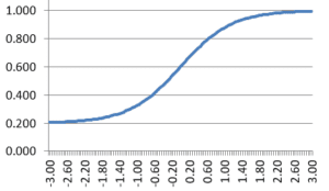
These parameters are used to graphically display an item response function (IRF), which models the probability of a correct answer as a function of ability.  An example IRF is below.  Here, the a parameter is approximately, 1.0, indicating a fairly discriminating test item.  The b parameter is approximately 0.0 (the point on the x-axis where the midpoint of the curve is), indicating an average-difficulty item; examinees of average ability would have a 60% chance of answering correctly.  The c parameter is approximately 0.20, like a 5-option multiple choice item.

Item response function

What does this mean conceptually?  We are trying to model the interaction of an examinee responding to an item, hence the name item response theory. Consider the x-axis to be z-scores on a standard normal scale.  Examinees with higher ability are much more likely to respond correctly.  Someone at +2.0 (97th percentile) has about a 94% chance of getting the item correct.  Meanwhile, someone at -2.0 has only a 37% chance.

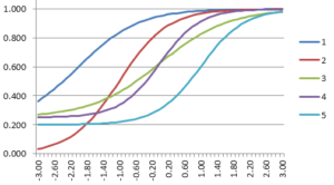
Of course, the parameters can and should differ from item to item, reflecting differences in item performance.  The following graph shows five IRFs.  The dark blue line is the easiest item, with a b of -2.00.  The light blue item is the hardest, with a b of +1.80.  The purple one has a c=0.00 while the light blue has c=0.25, indicating that it is susceptible to guessing.

five item response functions

These IRFs are not just a pretty graph or a way to describe how an item performs.  They are the basic building block to accomplishing those important goals mentioned earlier.  That comes next…


Applications of IRT to Improve Assessment

Item response theory uses the IRF for several purposes.  Here are a few.

  1. Interpreting and improving item performance
  2. Scoring examinees with maximum likelihood or Bayesian methods
  3. Form assembly, including linear on the fly testing (LOFT) and pre-equating
  4. Calculating the accuracy of examinee scores
  5. Development of computerized adaptive tests (CAT)
  6. Post-equating
  7. Differential item functioning (finding bias)
  8. Data forensics to find cheaters or other issues

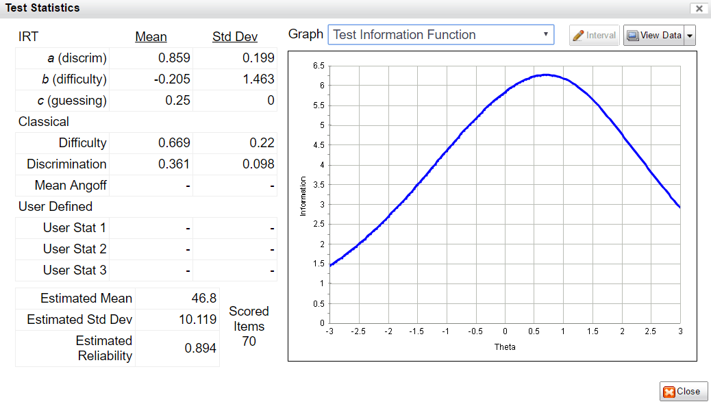
In addition to being used to evaluate each item individually, IRFs are combined in various ways to evaluate the overall test or form.  The two most important approaches are the conditional standard error of measurement (CSEM) and the test information function (TIF).  The test information function is higher where the test is providing more measurement information about examinees; if relatively low in a certain range of examinee ability, those examinees are not being measured accurately.  The CSEM is the inverse of the TIF, and has the interpretable advantage of being usable for confidence intervals; a person’s score plus or minus 1.96 times the SEM is a 95% confidence interval for their score.  The graph on the right shows part of the form assembly process in our  FastTest  platform.

test information function from item response theory


Advantages and Benefits of Item Response Theory

So why does this matter?  Let’s go back to the problems with classical test theory.  Why is IRT better?

  • Sample-independence of scale: Classical statistics are all sample dependent, and unusable on a different sample; results from IRT are sample-independent. within a linear transformation.  Two samples of different ability levels can be easily converted onto the same scale.
  • Test statistics: Classical statistics are tied to a specific test form.
  • Sparse matrices are OK: Classical test statistics do not work with sparse matrices introduced by multiple forms, linear on the fly testing, or adaptive testing.
  • Linking/equating: Item response theory has much stronger equating, so if your exam has multiple forms, or if you deliver twice per year with a new form, you can have much greater validity in the comparability of scores.
  • Measuring the range of students: Classical tests are built for the average student, and do not measure high or low students very well; conversely, statistics for very difficult or easy items are suspect.
  • Vertical scaling: IRT can do vertical scaling but CTT cannot.
  • Lack of accounting for guessing: CTT does not account for guessing on multiple choice exams.
  • Scoring: Scoring in classical test theory does not take into account item difficulty.  With IRT, you can score a student on any set of items and be sure it is on the same latent scale.
  • Adaptive testing: CTT does not support adaptive testing in most cases.  Adaptive testing has its own list of benefits.
  • Characterization of error: CTT assumes that every examinee has the same amount of error in their score (SEM); IRT recognizes that if the test is all middle-difficulty items, then low or high students will have inaccurate scores.
  • Stronger form building: IRT has functionality to build forms to be more strongly equivalent and meet the purposes of the exam.
  • Nonlinear function: IRT does not assume linear function of the student-item relationship when it is impossible.  CTT assumes a linear function (point-biserial) when it is blatantly impossible.

One Big Happy Family

Remember: Item response theory is actually a family of models, making flexible use of the parameters.  In some cases, only two (a,b) or one parameters (b) are used, depending on the type of assessment and fit of the data.  If there are multipoint items, such as Likert rating scales or partial credit items, the models are extended to include additional parameters. Learn more about the partial credit situation here.

Here’s a quick breakdown of the family tree, with the most common models.

Where can I learn more?

For more information, we recommend the textbook Item Response Theory for Psychologists by Embretson & Riese (2000) for those interested in a less mathematical treatment, or de Ayala (2009) for a more mathematical treatment.  If you really want to dive in, you can try the 3-volume Handbook of Item Response Theory edited by van der Linden, which contains a chapter discussing ASC’s IRT analysis software,  Xcalibre.

Want to talk to one of our experts about how to apply IRT?  Get in touch!

TALK TO US Contact

If you are delivering high-stakes tests in linear forms – or piloting a bank for CAT/LOFT – you are faced with the issue of how to equate the forms together.  That is, how can we defensibly translate a score on Form A to a score on Form B?  While the concept is simple, the methodology can be complex, and there is an entire area of psychometric research devoted to this topic. There are a number of ways to approach this issue, and IRT equating is the strongest.

Why do we need equating?

The need is obvious: to adjust for differences in difficulty to ensure that all examinees receive a fair score on a stable scale.  Suppose you take Form A and get s score of 72/100 while your friend takes Form B and gets a score of 74/100.  Is your friend smarter than you, or did his form happen to have easier questions?  Well, if the test designers built-in some overlap, we can answer this question empirically.

Suppose the two forms overlap by 50 items, called anchor items or equator items.  Both forms are each delivered to a large, representative sample. Here are the results.

Form Mean score on 50 overlap items Mean score on 100 total items
A 30 72
B 30 74

Because the mean score on the anchor items was higher, we then think that the Form B group was a little smarter, which led to a higher total score.

Now suppose these are the results:

Form Mean score on 50 overlap items Mean score on 100 total items
A 32 72
B 32 74

Now, we have evidence that the groups are of equal ability.  The higher total score on Form B must then be because the unique items on that form are a bit easier.

How do I calculate an equating?

You can equate forms with classical test theory (CTT) or item response theory (IRT).  However, one of the reasons that IRT was invented was that equating with CTT was very weak.  CTT methods include Tucker, Levine, and equipercentile.  Right now, though, let’s focus on IRT.

IRT equating

There are three general approaches to IRT equating.  All of them can be accomplished with our industry-leading software Xcalibre, though conversion equating requires an additional software called IRTEQ.

  1. Conversion
  2. Concurrent Calibration
  3. Fixed Anchor Calibration

Conversion

With this approach, you need to calibrate each form of your test using IRT, completely separately.  We then evaluate the relationship between IRT parameters on each form and use that to estimate the relationship to convert examinee scores.  Theoretically what you do is line up the IRT parameters of the common items and perform a linear regression, so you can then apply that linear conversion to scores.

But DO NOT just do a regular linear regression.  There are specific methods you must use, including mean/mean, mean/sigma, Stocking & Lord, and Haebara.  Fortunately, you don’t have to figure out all the calculations yourself, as there is free software available to do it for you: IRTEQ.

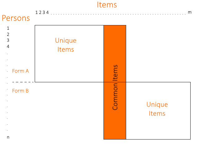
Concurrent Calibrationcommon item linking irt equating

The second approach is to combine the datasets into what is known as a sparse matrix.  You then run this single data set through the IRT calibration, and it will place all items and examinees onto a common scale.  The concept of a sparse matrix is typically represented by the figure below, representing the non-equivalent anchor test (NEAT) design approach.

The IRT calibration software will automatically equate the two forms and you can use the resultant scores.

Fixed Anchor Calibration

The third approach is a combination of the two above; it utilizes the separate calibration concept but still uses the IRT calibration process to perform the equating rather than separate software.

With this approach, you would first calibrate your data for Form A.  You then find all the IRT item parameters for the common items and input them into your IRT calibration software when you calibrate Form B.

You can tell the software to “fix” the item parameters so that those particular ones (from the common items) do not change.  Then all the item parameters for the unique items are forced onto the scale of the common items, which of course is the underlying scale from Form A.  This then also forces the scores from the Form B students onto the Form A scale.

How do these IRT equating approaches compare to each other?
concurrent calibration irt equating linking

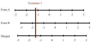
Concurrent calibration is arguably the easiest but has the drawback that it merges the scales of each form into a new scale somewhere in the middle.  If you need to report the scores on either form on the original scale, then you must use the Conversion or Fixed Anchor approaches.  This situation commonly happens if you are equating across time periods.

Suppose you delivered Form A last year and are now trying to equate Form B.  You can’t just create a new scale and thereby nullify all the scores you reported last year.  You must map Form B onto Form A so that this year’s scores are reported on last year’s scale and everyone’s scores will be consistent.

Where do I go from here?

If you want to do IRT equating, you need IRT calibration software.  All three approaches use it.  I highly recommend Xcalibre since it is easy to use and automatically creates reports in Word for you.  If you want to learn more about the topic of equating, the classic reference is the book by Kolen and Brennan (2004; 2014).  There are other resources more readily available on the internet, like this free handbook from CCSSO.  If you would like to learn more about IRT, I recommend the books by de Ayala (2008) and Embretson & Reise (2000).  An intro is available in our blog post.