Posts on psychometrics: The Science of Assessment

Sympson-Hetter is a method of item exposure control within the algorithm of Computerized adaptive testing (CAT).  It prevents the algorithm from over-using the best items in the pool.

CAT is a powerful paradigm for delivering tests that are smarter, faster, and fairer than the traditional linear approach.  However, CAT is not without its challenges.  One is that it is a greedy algorithm that always selects your best items from the pool if it can.  The way that CAT researchers address this issue is with item exposure controls.  These are sub algorithms that are injected into the main item selection algorithm, to alter it from always using the best items. The Sympson-Hetter method is one such approach.  Another is the Randomesque method.

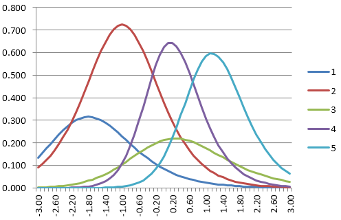
The Randomesque Method5 item information functions IIF for Sympson-Hetter

The simplest approach is called the randomesque method.  This selects from the top X items in terms of item information (a term from item response theory), usually for the first Y items in a test.  For example, instead of always selecting the top item, the algorithm finds the 3 top items and then randomly selects between those.

The figure on the right displays item information functions (IIFs) for a pool of 5 items.  Suppose an examinee had a theta estimate of 1.40.  The 3 items with the highest information are the light blue, purple, and green lines (5, 4, 3).  The algorithm would first identify this and randomly pick amongst those three.  Without item exposure controls, it would always select Item 4.

The Sympson-Hetter Method

A more sophisticated method is the Sympson-Hetter method.

Here, the user specifies a target proportion as a parameter for the selection algorithm.  For example, we might decide that we do not want an item seen by more than 75% of examinees.  So, every time that the CAT algorithm goes into the item pool to select a new item, we generate a random number between 0 and 1, which is then compared to the threshold.  If the number is between 0 and 0.75 in this case, we go ahead and administer the item.  If the number is from 0.75 to 1.0, we skip over it and go on to the next most informative item in the pool, though we then do the same comparison for that item.

Why do this?  It obviously limits the exposure of the item.  But just how much it limits it depends on the difficulty of the item.  A very difficult item is likely only going to be a candidate for selection for very high-ability examinees.  Let’s say it’s the top 4%… well, then the approach above will limit it to 3% of the sample overall, but 75% of the examinees in its neighborhood.

On the other hand, an item of middle difficulty is used not only for middle examinees but often for any examinee.  Remember, unless there are some controls, the first item for the test will be the same for everyone!  So if we apply the Sympson-Hetter rule to that item, it limits it to 75% exposure in a more absolute sense.

Because of this, you don’t have to set that threshold parameter to the same value for each item.  The original recommendation was to do some CAT simulation studies, then set the parameters thoughtfully for different items.  Items that are likely to be highly exposed (middle difficulty with high discrimination) might deserve a more strict parameter like 0.40.  On the other hand, that super-difficult item isn’t an exposure concern because only the top 4% of students see it anyway… so we might leave its parameter at 1.0 and therefore not limit it at all.

Is this the only method available?

No.  As mentioned, there’s that simple randomesque approach.  But there are plenty more.  You might be interested in this paper, this paper, or this paper.  The last one reviews the research literature from 1983 to 2005.

What is the original reference?

Sympson, J. B., & Hetter, R. D. (1985, October). Controlling item-exposure rates in computerized adaptive testing. Proceedings of the 27th annual meeting of the Military Testing Association (pp. 973–977). San Diego, CA: Navy Personnel Research and Development Center.

How can I apply this to my tests?

Well, you certainly need a CAT platform first.  Our platform at ASC allows this method right out of the box – that is, all you need to do is enter the target proportion when you publish your exam, and the Sympson-Hetter method will be implemented.  No need to write any code yourself!  Click here to sign up for a free account.

A test security plan (TSP) is a document that lays out how an assessment organization address security of its intellectual property, to protect the validity of the exam scores.  If a test is compromised, the scores become meaningless, so security is obviously important.  The test security plan helps an organization anticipate test security issues, establish deterrent and detection methods, and plan responses.  It can also include validity threats not security-related, such as how to deal with examinees that have low motivation.  Note that it is not limited to delivery; it can often include topics like how to manage item writers.

Since the first tests were developed 2000 years ago for entry into the civil service of Imperial China, test security has been a concern.  The reason is quite straightforward: most threats to test security are also validity threats. The decisions we make with test scores could therefore be invalid, or at least suboptimal.  It is therefore imperative that organizations that use or develop tests should develop a TSP. 

There are several reasons to develop a test security plan.  First, it drives greater security and therefore validity.  The TSP will enhance the legal defensibility of the testing program.  It helps to safeguard the content, which is typically an expensive investment for any organization that develops tests themselves.  If incidents do happen, they can be dealt with more swiftly and effectively.  It helps to manage all the security-related efforts.

The development of such a complex document requires a strong framework.  We advocate a framework with three phases: planning, implementation, and response.  In addition, the TSP should be revised periodically.

Phase 1: Planning

The first step in this phase is to list all potential threats to each assessment program at your organization.  This could include harvesting of test content, preknowledge of test content from past harvesters, copying other examinees, proxy testers, proctor help, and outside help.  Next, these should be rated on axes that are important to the organization; a simple approach would be to rate on potential impact to score validity, cost to the organization, and likelihood of occurrence.  This risk assessment exercise will help the remainder of the framework.

Next, the organization should develop the test security plan.  The first piece is to identify deterrents and procedures to reduce the possibility of issues.  This includes delivery procedures (such as a lockdown browser or proctoring), proctor training manuals, a strong candidate agreement, anonymous reporting pathways, confirmation testing, and candidate identification requirements.  The second piece is to explicitly plan for psychometric forensics. 

This can range from complex collusion indices based on item response theory to simple flags, such as a candidate responding to a certain multiple choice option more than 50% of the time or obtaining a score in the top 10% but in the lowest 10% of time.  The third piece is to establish planned responses.  What will you do if a proctor reports that two candidates were copying each other?  What if someone obtains a high score in an unreasonably short time? 

What if someone obviously did not try to pass the exam, but still sat there for the allotted time?  If a candidate were to lose a job opportunity due to your response, it helps you defensibility to show that the process was established ahead of time with the input of important stakeholders.

Phase 2: Implementation

The second phase is to implement the relevant aspects of the Test Security Plan, such as training all proctors in accordance with the manual and login procedures, setting IP address limits, or ensuring that a new secure testing platform with lockdown is rolled out to all testing locations.  There are generally two approaches.  Proactive approaches attempt to reduce the likelihood of issues in the first place, and reactive methods happen after the test is given.  The reactive methods can be observational, quantitative, or content-focused.  Observational methods include proctor reports or an anonymous tip line.  Quantitative methods include psychometric forensics, for which you will need software like SIFT.  Content-focused methods include automated web crawling.

Both approaches require continuous attention.  You might need to train new proctors several times per year, or update your lockdown browser.  If you use a virtual proctoring service based on record-and-review, flagged candidates must be periodically reviewed.  The reactive methods are similar: incoming anonymous tips or proctor reports must be dealt with at any given time.  The least continuous aspect is some of the psychometric forensics, which depend on a large-scale data analysis; for example, you might gather data from tens of thousands of examinees in a testing window and can only do a complete analysis at that point, which could take several weeks.

Phase 3: Response

The third phase, of course, to put your planned responses into motion if issues are detected.  Some of these could be relatively innocuous; if a proctor is reported as not following procedures, they might need some remedial training, and it’s certainly possible that no security breach occurred.  The more dramatic responses include actions taken against the candidate.  The most lenient is to provide a warning or simply ask them to retake the test.  The most extreme methods include a full invalidation of the score with future sanctions, such as a five-year ban on taking the test again, which could prevent someone from entering a profession for which they spent 8 years and hundreds of thousands of dollars in educative preparation.

What does a test security plan mean for me?

It is clear that test security threats are also validity threats, and that the extensive (and expensive!) measures warrant a strategic and proactive approach in many situations.  A framework like the one advocated here will help organizations identify and prioritize threats so that the measures are appropriate for a given program.  Note that the results can be quite different if an organization has multiple programs, from a practice test to an entry level screening test to a promotional test to a professional certification or licensure.

Another important difference between test sponsors/publishers and test consumers.  In the case of an organization that purchases off-the-shelf pre-employment tests, the validity of score interpretations is of more direct concern, while the theft of content might not be an immediate concern.  Conversely, the publisher of such tests has invested heavily in the content and could be massively impacted by theft, while the copying of two examinees in the hiring organization is not of immediate concern.

In summary, there are more security threats, deterrents, procedures, and psychometric forensic methods than can be discussed in one blog post, so the focus here rather on the framework itself.  For starters, start thinking strategically about test security and how it impacts their assessment programs by using the multi-axis rating approach, then begin to develop a Test Security Plan.  The end goal is to improve the health and validity of your assessments.


Want to implement some of the security aspects discussed here, like online delivery lockdown browser, IP address limits, and proctor passwords?

Sign up for a free account in FastTest!

The standard error of measurement (SEM) is one of the core concepts in psychometrics.  One of the primary assumptions of any assessment is that it is accurately and consistently measuring whatever it is we want to measure.  We, therefore, need to demonstrate that it is doing so.  There are a number of ways of quantifying this, and one of the most common is the SEM.

The SEM can be used in both the classical test theory (CTT) perspective and item response theory (IRT) perspective, though it is defined quite differently in both.

The Standard Error of Measurement in Classical Test Theory

In CTT, it is defined as

SEM = SD*sqrt(1-r),

where SD is the standard deviation of scores for everyone who took the test, and r is the reliability of the test.  It is interpreted as the standard deviation of scores that you would find if you had the person take the test over and over, with a fresh mind each time.  A confidence interval with this is then interpreted as the band where you would expect the person’s true score on the test to fall.

This has some conceptual disadvantages.  For one, it assumes that SEM is the same for all examinees, which is unrealistic.  The interpretation focuses only on this single test form rather than the accuracy of measuring someone’s true standing on the trait.  Moreover, it does not utilize the examinee’s responses in any way.  Lord (1984) suggested a conditional standard error of measurement based on classical test theory, but it focuses on the error of the examinee taking the same test again, rather than the measurement of the true latent value as is done with IRT below.

The classical SEM is reported in Iteman for each subscore, the total score, score on scored items only, and score on pretest items.

The Standard Error of Measurement in Item Response Theoryconditional standard error of measurement

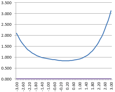
The weaknesses of the classical SEM are one of the reasons that IRT was developed.  IRT conceptualizes the SEM as a continuous function across the range of student ability, which is an inversion of the test information function (TIF).  A test form will have more accuracy – less error – in a range of ability where there are more items or items of higher quality.  That is, a test with most items of middle difficulty will produce accurate scores in the middle of the range, but not measure students on the top or bottom very well.  The example below is a test that has many items below the average examinee score (θ) of 0.0 so that any examinee with a score above 1.0 has a relatively inaccurate score, namely with an SEM greater than 0.25.

This is actually only the predicted SEM based on all the items in a test/pool.  The observed SEM can differ for each examinee based on the items that they answered, and which ones they answered correctly.  If you want to calculate the IRT SEM on a test of yours, you need to download Xcalibre and implement a full IRT calibration study.

The standard error of the mean is one of the three main standard errors in psychometrics and psychology.  Its purpose is to help conceptualize the error in estimating the mean of some population based on a sample.  The SEM is a well-known concept from the general field of statistics, used in an untold number of applications.

For example, a biologist might catch a number of fish from a lake, measure their length, and use that data to determine the average size of fish in the lake.  In psychometrics and psychology, we usually utilize data from some measurement of people.

For example, suppose we have a population of 5 employees with scores below on a 10 item assessment on safety procedures.

Student  Score

1             4

2             6

3             6

4             8

5             7

Then let’s suppose we are drawing a sample of 4.  There are 5 different ways to do this, but let’s just say it’s the first 4.  The average score is (4+6+6+8)/4=6, and the standard deviation for the sample is 1.63.  The standard error of the mean says that

   SEM=SD/sqrt(n) = 1.63/sqrt(4) = 0.815.

Because a 95% confidence interval is 1.96 standard errors around the average, and the average is 6, this says we expect the true mean of the distribution to be somewhere between 4.40 to 7.60.  Obviously, this is not very exact!  There are two reasons for that in this case: the SD is relatively large 1.63 on a scale of 0 to 10, and the N is only 4.  If you had a sample N of 10,000, for example, you’d be dividing the 1.63 by 100, leading to an SEM of only 0.0163.

How is this useful?  Well, this tells us that even the wide range of 4.40 to 7.60 means that the average score is fairly low; that our employees probably need some training on safety procedures.  The other two standard errors in psychology/psychometrics are more complex and more useful, though.  I’ll be covering those in future posts.

One of my graduate school mentors once said in class that there are three standard errors that everyone in the assessment or I/O Psych field needs to know: mean, error, and estimate.  They are quite distinct in concept and application but easily confused by someone with minimal training.

I’ve personally seen the standard error of the mean reported as the standard error of measurement, which is completely unacceptable.

So in this post, I’ll briefly describe each so that the differences are clear.  In later posts, I’ll delve deeper into each of the standard errors.


Standard Error of the Mean

This is the standard error that you learned about in Introduction to Statistics back in your sophomore year of college/university.  It is related to the Central Limit Theorem, the cornerstone of statistics.  Its purpose is to provide an index of accuracy (or conversely, error) in a sample mean.  Any sample drawn from a population will have an average, but these can vary.  The standard error of the mean estimates the variation we might expect in these different means from different samples and is defined as

   SEmean = SD/sqrt(n)

Where SD is the sample’s standard deviation and n is the number of observations in the sample.  This can be used to create a confidence interval for the true population mean.

The most important thing to note, with respect to psychometrics, is that this has nothing to do with psychometrics.  This is just general statistics.  You could be weighing a bunch of hay bales and calculating their average; anything where you are making observations.  It can be used, however, with assessment data.

For example, if you do not want to make every student in a country take a test, and instead sample 50,000 students, with a mean of 71 items correct with an SD of 12.3, then the SEM is  12.3/sqrt(50000) = 0.055.  You can be 95% certain that the true population means then lies in the narrow range of 71 +- 0.055.

Click here to read more.

Standard Error of Measurement

More important in the world of assessment is the standard error of measurement.  Its purpose is to provide an index of the accuracy of a person’s score on a test.  That is a single person, rather than a group like with the standard error of the mean.  It can be used in both the classical test theory perspective and item response theory perspective, though it is defined quite differently in both.

In classical test theory, it is defined as

   SEM = SD*sqrt(1-r)

Where SD is the standard deviation of scores for everyone who took the test, and r is the reliability of the test.  It can be interpreted as the standard deviation of scores that you would find if you had the person take the test over and over, with a fresh mind each time.  A confidence interval with this is then interpreted as the band where you would expect the person’s true score on the test to fall.

Item Response Theory conceptualizes the SEM as a continuous function across the range of student abilities.  A test form will have more accuracy – less error – in a range of abilities where there are more items or items of higher quality.  That is, a test with most items of middle difficulty will produce accurate scores in the middle of the range, but not measure students on the top or bottom very well.  The example below is a test that has many items above the average examinee score (θ) of 0.0 so that any examinee with a score of less than 0.0 has a relatively inaccurate score, namely with an SEM greater than 0.50.


Standard error of measurement and test information function

For a deeper discussion of SEM, click here.


Standard Error of the Estimate

Lastly, we have the standard error of the estimate.  This is an estimate of the accuracy of a prediction that is made, usually in the paradigm of linear regression.  Suppose we are using scores on a 40 item job knowledge test to predict job performance, and we have data on a sample of 1,000 job incumbents that took the test last year and have job performance ratings from this year on a measure that entails 20 items scored on a 5 point scale for a total of 100 points.

There might have been 86 incumbents that scored 30/40 on the test, and they will have a range of job performance, let’s say from 61 to 89.  If a new person takes the test and scores 30/40, how would we predict their job performance?

The SEE is defined as

       SEE = SDy*sqrt(1-r2)

Here, the r is the correlation of x and y, not reliability. Many statistical packages can estimate linear regression, SEE, and many other related statistics for you.  In fact, Microsoft Excel comes with a free package to implement simple linear regression.  Excel estimates the SEE as 4.69 in the example above, and the regression slope and intercept are 29.93 and 1.76, respectively

Given this, we can estimate the job performance of a person with a 30 test score to be 82.73.  A 95% confidence interval for a candidate with a test score of 30 is then 82.71-(4.69*1.96) to 82.71+(4.69*1.96), or 73.52 to 91.90.

You can see how this might be useful in prediction situations.  Suppose we wanted to be sure that we only hired people who are likely to have a job performance rating of 80 or better?  Well, a cutscore of 30 on the test is therefore quite feasible.


OK, so now what?

Well, remember that these three standard errors are quite different and are not even in related situations.  When you see a standard error requested – for example if you must report the standard error for an assessment – make sure you use the right one!

Validity, in its modern conceptualization, refers to evidence that supports our intended interpretations of test scores (see Chapter 1 of APA/AERA/NCME Standards for full treatment).  Validity threats are issues that hinder the interpretations and use of scores.  The word “interpretation” is key because test scores can be interpreted in different ways, including ways that are not intended by the test designers.

For example, a test given at the end of Nursing school to prepare for a national licensure exam might be used by the school as a sort of Final Exam.  However, the test was not designed for this purpose and might not even be aligned with the school’s curriculum.

Another example is that certification tests are usually designed to demonstrate minimal competence, not differentiate amongst experts, so interpreting a high score as expertise might not be warranted.

Validity threats: Always be on the lookout!

Test sponsors, therefore, must be vigilant against any validity threats.  Some of these, like the two aforementioned examples, might be outside the scope of the organization.  While it is certainly worthwhile to address such issues, our primary focus is on aspects of the exam itself.

Which validity threats rise to the surface in psychometric forensics?

Here, we will discuss several threats to validity that typically present themselves in psychometric forensics, with a focus on security aspects.  However, I’m not just listing security threats here, as psychometric forensics is excellent at flagging other types of validity threats too.

Threat Description Approach Example Indices
Collusion (copying) Examinees are copying answers from one another, usually with a defined Source. Error similarity (only looks at incorrect) 2 examinees get the same 10 items wrong, and select the same distractor on each B-B Ran, B-B Obs, K, K1, K2, S2
Response similarity 2 examinees give the same response on 98/100 items S2, g2, ω, Zjk
Group level help/issues Similar to collusion but at a group level; could be examinees working together, or receiving answers from a teacher/proctor.  Note that many examinees using the same brain dump would have a similar signature but across locations. Group level statistics Location has one of the highest mean scores but lowest mean times Descriptive statistics such as mean score, mean time, and pass rate
Response or error similarity On a certain group of items, the entire classroom gives the same answers Roll-up analysis, such as mean collusion flags per group; also erasure analysis (paper only)
Pre-Knowledge Examinee comes in to take the test already knowing the items and answers, often purchased from a brain dump website. Time-Score analysis Examinee has high score and very short time RTE or total time vs. scores
Response or error similarity Examinee has all the same responses as a known brain dump site All indices
Pretest item comparison Examinee gets 100% on existing items but 50% on new items Pre vs Scored results
Person fit Examinee gets the 10 hardest items correct but performs below average on the rest of the items Guttman indices, lz
Harvesting Examinee is not actually taking the test, but is sitting it to memorize items so they can be sold afterwards, often at a brain dump website.  Similar signature to Sleepers but more likely to occur on voluntary tests, or where high scores benefit examinees. Time-Score analysis Low score, high time, few attempts. RTE or total time vs. scores
Mean vs Median item time Examinee “camps” on 10 items to memorize them; mean item time much higher than the median Mean-Median index
Option flagging Examinee answers “C” to all items in the second half Option proportions
Low motivation: Sleeper Examinees are disengaged, producing data that is flagged as unusual and invalid; fortunately, not usually a security concern but could be a policy concern. Similar signature to Harvester but more likely to occur on mandatory tests, or where high scores do not benefit examinees. Time-Score analysis Low score, high time, few attempts. RTE or total time vs. scores
Item timeout rate If you have item time limits, examinee hits them Proportion items that hit limit
Person fit Examinee attempt a few items, passes through the rest Guttman indices, lz
Low motivation: Clicker Examinees are disengaged, producing data that is flagged as unusual and invalid; fortunately, not usually a security concern but could be a policy concern. Similar idea to Sleeper but data is quite different. Time-Score analysis Examinee quickly clicks “A” to all items, finishing with a low time and low score RTE, Total time vs. scores
Option flagging See above Option proportions

One of the core concepts in psychometrics is item difficulty.  This refers to the probability that examinees will get the item correct for educational/cognitive assessments or respond in the keyed direction with psychological/survey assessments (more on that later).  Difficulty is important for evaluating the characteristics of an item and whether it should continue to be part of the assessment; in many cases, items are deleted if they are too easy or too hard.  It also allows us to better understand how the items and test as a whole operate as a measurement instrument, and what they can tell us about examinees.

I’ve heard of “item facility.” Is that similar?

Item difficulty is also called item facility, which is actually a more appropriate name.  Why?  The P value is a reverse of the concept: a low value indicates high difficulty, and vice versa.  If we think of the concept as facility or easiness, then the P value aligns with the concept; a high value means high easiness.  Of course, it’s hard to break with tradition, and almost everyone still calls it difficulty.  But it might help you here to think of it as “easiness.”

How do we calculate classical item difficulty?

There are two predominant paradigms in psychometrics: classical test theory (CTT) and item response theory (IRT).  Here, I will just focus on the simpler approach, CTT.

To calculate classical item difficulty with dichotomous items, you simply count the number of examinees that responded correctly (or in the keyed direction) and divide by the number of respondents.  This gets you a proportion, which is like a percentage but is on the scale of 0 to 1 rather than 0 to 100.  Therefore, the possible range that you will see reported is 0 to 1.  Consider this data set.

Person Item1 Item2 Item3 Item4 Item5 Item6 Score
1 0 0 0 0 0 1 1
2 0 0 0 0 1 1 2
3 0 0 0 1 1 1 3
4 0 0 1 1 1 1 4
5 0 1 1 1 1 1 5
Diff: 0.00 0.20 0.40 0.60 0.80 1.00

Item6 has a high difficulty index, meaning that it is very easy.  Item4 and Item5 are typical items, where the majority of items are responding correctly.  Item1 is extremely difficult; no one got it right!

For polytomous items (items with more than one point), classical item difficulty is the mean response value.  That is, if we have a 5 point Likert item, and two people respond 4 and two response 5, then the average is 4.5.  This, of course, is mathematically equivalent to the P value if the points are 0 and 1 for a no/yes item.  An example of this situation is this data set:

Person Item1 Item2 Item3 Item4 Item5 Item6 Score
1 1 1 2 3 4 5 1
2 1 2 2 4 4 5 2
3 1 2 3 4 4 5 3
4 1 2 3 4 4 5 4
5 1 2 3 5 4 5 5
Diff: 1.00 1.80 2.60 4.00 4.00 5.00

Note that this is approach to calculating difficulty is sample-dependent.  If we had a different sample of people, the statistics could be quite different.  This is one of the primary drawbacks to classical test theory.  Item response theory tackles that issue with a different paradigm.  It also has an index with the right “direction” – high values mean high difficulty with IRT.

If you are working with multiple choice items, remember that while you might have 4 or 5 responses, you are still scoring the items as right/wrong.  Therefore, the data ends up being dichotomous 0/1.

Very important final note: this P value is NOT to be confused with p value from the world of hypothesis testing.  They have the same name, but otherwise are completely unrelated.  For this reason, some psychometricians call it P+ (pronounced “P-plus”), but that hasn’t caught on.

How do I interpret classical item difficulty?

For educational/cognitive assessments, difficulty refers to the probability that examinees will get the item correct.  If more examinees get the item correct, it has low difficulty.  For psychological/survey type data, difficulty refers to the probability of responding in the keyed direction.  That is, if you are assessing Extraversion, and the item is “I like to go to parties” then you are evaluating how many examinees agreed with the statement.

What is unique with survey type data is that it often includes reverse-keying; the same assessment might also have an item that is “I prefer to spend time with books rather than people” and an examinee disagreeing with that statement counts as a point towards the total score.

For the stereotypical educational/knowledge assessment, with 4 or 5 option multiple choice items, we use general guidelines like this for interpretation.

Range Interpretation Notes
0.0-0.3 Extremely difficult Examinees are at chance level or even below, so your item might be miskeyed or have other issues
0.3-0.5 Very difficult Items in this range will challenge even top examinees, and therefore might elicit complaints, but are typically very strong
0.5-0.7 Moderately difficult These items are fairly common, and a little on the tougher side
0.7-0.90 Moderately easy These are the most common range of items on most classically built tests; easy enough that examinees rarely complain
0.90-1.0 Very easy These items are mastered by most examinees; they are actually too easy to provide much info on examinees though, and can be detrimental to reliability.

Do I need to calculate this all myself?

No.  There is plenty of software to do it for you.  If you are new to psychometrics, I recommend CITAS, which is designed to get you up and running quickly but is too simple for advanced situations.  If you have large samples or are involved with production-level work, you need Iteman.  Sign up for a free account with the button below.  If that is you, I also recommend that you look into learning IRT if you have not yet.

It’s October 30, 2017, and collusion is all over the news today… but I want to talk about a different kind of collusion.  That is, non-independent test taking.  In the field of psychometric forensics, examinee collusion refers to cases where an examinee takes a test with some sort of external help in obtaining the correct answers.  There are several possibilities:

  1. Low ability examinees copy off a high ability examinee (known as the Source); could be unbeknownst to the source.
  2. Examinees work together and pool their answers.
  3. Examinees receive answers from a present third party, such as a friend outside with Bluetooth, a teacher, or a proctor.
  4. Multiple examinees obtaining answers from a brain dump site, known as preknowledge; while not strictly collusion, we’d likely find similar answer patterns in that group, even if they never met each other.

The research on the field has treated all of these more or less equivalently, and as a group.  I’d like to argue that we stop doing that.  Why? The data patterns can be different, and can therefore be detected (or not detected) by different types of forensics.  Most importantly, some collusion indices are designed specifically for some cases, and we need to treat them as such.  More broadly, perhaps we need a theoretical background on types of collusion – part of an even broader theory on types of invalid test-taking – as a basis to fit, evaluate, and develop indices.

What do I mean by this?  Well, some collusion indices are explicitly designed around the assumption that there is a Source and a copier(s).  The strongest examples are the K-variants (Sotaridona, 2003) and Wollack’s (1997) omega.  Other indices do not assume this, such as Bellezza & Bellezza (1989); they simply look for similarities in responses, either on errors alone or on both errors and correct answers.

Collusion indices, if you’re not familiar with them, evaluate each possible pair of examinees and look for similar response patterns; if you have 1000 examinees, there are (1000 x 9999)/2 = 4,999,500 pairs.  If you use an index that evaluates the two directions separately (Examinee 1 is Source and 2 is Copier, then 2 is Source and 1 is Copier), you are calculating the index 9,999,000 times on this relatively small data set.

Primary vs. Secondary Collusion

Consider the first case above, which is generally of interest.  I’d like to delineate the difference between primary collusion and secondary collusion.  Primary collusion is what we are truly trying to find: if examinees are copying off another examinee.  Some indices are great at finding this.  But there is also secondary collusion; if multiple examinees are copiers, they will also have very similar response patterns, though the data signature will be different than if paired with the Source.  Indices designed to find primary collusion might not be as strong as finding this; rightly so, you might argue.

The other three cases above, I’d argue, are also secondary collusion.  There is no true Source present in the examinees, but we are certainly going to find unusually similar response patterns.  Indices that are explicitly designed to find the Source are not going to have the statistical power that was intended.  They require a slightly different set of assumptions, different interpretations, and different calculations.

What might the different calculations be?  That’s for another time.  I’m currently working through a few ideas.  The most recent is based on the discovery that the highly regarded S2 index (Sotaridona, 2003) makes assumptions that are regularly violated in real data, and that the calculations need to be modified.  I’ll be integrating the new index into SIFT.

An example of examinee collusion

To demonstrate, I conducted a brief simulation study, part of a much larger study to be published at a future date.  I took a data set of a national educational assessment (N=16,666, 50 MC items), randomly selected 1,000 examinees, randomly assigned them to one of 10 locations, and then created a copying situation in one location.  To do this, I found the highest ability examinee at that location and the lowest 50, then made those low 50 copy the answers off the high examinee for the 25 hardest items.  This is a fairly extreme and clear-cut example, so we’d hope that the collusion indices pick up on such an obvious data signature.

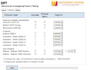
Let’s start by investigating that statement.  This is an evaluation of power, which is the strength of a statistical test to find something when something is actually there (though technically, not all of these indices are statistical tests).  We hope that we can find all 50 instances of primary collusion as well as most of the secondary collusion.  As of today, SIFT calculates 15 collusion indices; for a full description of these, download a free copy and check out the manual.

SIFT test security data forensics

What does this all mean?

Well, my original point was that we need to differentiate the Primary and Secondary cases of collusion, and evaluate them separately when we can.  An even broader point was that we need a specific framework on types of invalid test instances and the data signatures they each leave, but that’s worth an article on its own.

If the topic of index comparison is interesting to you, check out the chapter by Zopluogu (2016).  He also found the power for S2 to be low, and the Type I errors to be conservative, though the Type II were not reported there.  That research stemmed from a dissertation at the University of Minnesota, which probably has a fuller treatment; my goal here is not to fully repeat that extensive study, but to provide some interesting interpretations.

In the past decade, terms like machine learning, artificial intelligence, and data mining are becoming greater buzzwords as computing power, APIs, and the massively increased availability of data enable new technologies like self-driving cars. However, we’ve been using methodologies like machine learning in psychometrics for decades. So much of the hype is just hype.

So, what exactly is Machine Learning?

Unfortunately, there is no widely agreed-upon definition, and as Wikipedia notes, machine learning is often conflated with data mining. A broad definition from Wikipedia is that machine learning explores the study and construction of algorithms that can learn from and make predictions on data. It’s often divided into supervised learning, where a researcher drives the process, and unsupervised learning, where the computer is allowed to creatively run wild and look for patterns. The latter isn’t of much use to us, at least yet.

Supervised learning includes specific topics like regression, dimensionality reduction, anomaly detection that we obviously have in Psychometrics. But its the general definition above that really fits what Psychometrics has been doing for decades.

What is Machine Learning in Psychometrics?

We can’t cover all the ways that machine learning and related topics are used in psychometrics and test development, but here’s a sampling. My goal is not to cover them all but to point out that this is old news and that should not get hung up on buzzwords and fads and marketing schticks – but by all means, we should continue to drive in this direction.

Dimensionality Reduction

One of the first, and most straightforward, areas is dimensionality reduction. Given a bunch of unstructured data, how can we find some sort of underlying structure, especially based on latent dimension? We’ve been doing this, utilizing methods like cluster analysis and factor analysis, since Spearman first started investigating the structure of intelligence 100 years ago. In fact, Spearman helped invent those approaches to solve the problems that he was trying to address in psychometrics, which was a new field at the time and had no methodology yet. How seminal was this work in psychometrics for the field of machine learning in general? The Coursera MOOC on Machine Learning uses Spearman’s work as an example in one of the early lectures!

Classification

Classification is a typical problem in machine learning. A common example is classifying images, and the classic dataset is the MNIST handwriting set (though Silicon Valley fans will think of the “not hot dog” algorithm). Given a bunch of input data (image files) and labels (what number is in the image), we develop an algorithm that most effectively can predict future image classification.  A closer example to our world is the iris dataset, where several quantitative measurements are used to predict the species of a flower.

The contrasting groups method of setting a test cutscore is a simple example of classification in psychometrics. We have a training set where examinees are already classified as pass/fail by a criterion other than test score (which of course rarely happens, but that’s another story), and use mathematical models to find the cutscore that most efficiently divides them. Not all standard setting methods take a purely statistical approach; understandably, the cutscores cannot be decided by an arbitrary computer algorithm like support vector machines or they’d be subject to immediate litigation. Strong use of subject matter experts and integration of the content itself is typically necessary.

Of course, all tests that seek to assign examinees into categories like Pass/Fail are addressing the classification problem. Some of my earliest psychometric work on the sequential probability ratio test and the generalized likelihood ratio was in this area.

One of the best examples of supervised learning for classification, but much more advanced than the contrasting groups method, is automated essay scoring, which as been around for about 2 decades. It has all the classic trappings: a training set where the observations are classified by humans first, and then mathematical models are trained to best approximate the humans. What makes it more complex is that the predictor data is now long strings of text (student essays) rather than a single number.

Anomaly Detection

The most obvious way this is used in our field is psychometric forensics, trying to find examinees that are cheating or some other behavior that warrants attention. But we also use it to evaluate model fit, possibly removing items or examinees from our data set.

Using Algorithms to Learn/Predict from Data

Item response theory is a great example of the general definition. With IRT, we are certainly using a training set, which we call a calibration sample. We use it to train some models, which are then used to make decisions in future observations, primarily scoring examinees that take the test by predicting where those examinees would fall in the score distribution of the calibration sample. IRT is also applied to solve more sophisticated algorithmic problems: Computerized adaptive testing and automated test assembly are fantastic examples. We IRT more generally to learn from the data; which items are most effective, which are not, the ability range where the test provides most precision, etc.

What differs from the Classification problem is that we don’t have a “true state” of labels for our training set. That is, we don’t know what the true scores are of the examinees, or if they are truly a “pass” or a “fail” – especially because those terms can be somewhat arbitrary. It is for this reason we rely on a well-defined model with theoretical reasons for it fitting our data, rather than just letting a machine learning toolkit analyze it with any model it feels like.

Arguably, classical test theory also fits this definition. We have a very specific mathematical model that is used to learn from the data, including which items are stronger or more difficult than others, and how to construct test forms to be statistically equivalent. However, its use of prediction is much weaker. We do not predict where future examinees would fall in the distribution of our calibration set. The fact that it is test-form-specific hampers is generalizability.

Reinforcement learning

The Wikipedia article also mentions reinforcement learning. This is used less often in psychometrics because test forms are typically published with some sort of finality. That is, they might be used in the field for a year or two before being retired, and no data is analyzed in that time except perhaps some high level checks like the NCCA Annual Statistical Report. Online IRT calibration is a great example, but is rarely used in practice. There, response data is analyzed algorithmically over time, and used to estimate or update the IRT parameters. Evaluation of parameter drift also fits in this definition.

Use of Test Scores

We also use test scores “outside” the test in a machine learning approach. A classic example of this is using pre-employment test scores to predict job performance, especially with additional variables to increase the incremental validity. But I’m not going to delve into that topic here.

Automation

Another huge opportunity for machine learning in psychometrics that is highly related is automation. That is, programming computers to do tasks more effectively or efficient than humans. Automated test assembly and automated essay scoring are examples of this, but there are plenty of of ways that automation can help that are less “cool” but have more impact. My favorite is the creation of psychometrics reports; Iteman and Xcalibre do not produce any numbers also available in other software, but they automatically build you a draft report in MS Word, with all the tables, graphs, and narratives already embedded. Very unique. Without that automation, organizations would typically pay a PhD psychometrician to spend hours of time on copy-and-paste, which is an absolute shame. The goal of my mentor, Prof. David Weiss, and myself is to automate the test development cycle as a whole; driving job analysis, test design, item writing, item review, standard setting, form assembly, test publishing, test delivery, and scoring. There’s no reason people should be allowed to continue making bad tests, and then using those tests to ruin people’s lives, when we know so much about what makes a decent test.

Summary

I am sure there are other areas of psychometrics and the testing industry that are soon to be disrupted by technological innovations such as this. What’s next?

As this article notes, the future direction is about the systems being able to learn on their own rather than being programmed; that is, more towards unsupervised learning than supervised learning. I’m not sure how well that fits with psychometrics.

But back to my original point: psychometrics has been a data-driven field since its inception a century ago. In fact, we contributed some of the methodology that is used generally in the field of machine learning and data analytics. So it shouldn’t be any big news when you hear terms like machine learning, data mining, AI, or dimensionality reduction used in our field! In contrast, I think it’s more important to consider how we remove roadblocks to more widespread use.

One of the hurdles we need to overcome for machine learning in psychometrics yet is simply how to get more organizations doing what has been considered best practice for decades. There are two types of problem organizations. The first type is one that does not have the sample sizes or budget to deal with methodologies like I’ve discussed here. The salient example I always think of is a state licensure test required by law for a niche profession that might have only 3 examinees per year (I have talked with such programs!). Not much we can do there. The second type is those organizations that indeed have large sample sizes and a decent budget, but are still doing things the same way they did them 30 years ago. How can we bring modern methods and innovations to these organizations? Because they will definitely only make their tests more effective and fairer.
An emerging sector in the field of psychometrics is the area devoted to analyzing test data to find cheaters and other illicit or invalid testing behavior. We lack a generally agreed-upon and marketable term for that sort of work, and I’d like to suggest that we use Psychometric Forensics.

While research on this topic is more than 50 years old, the modern era did not begin until Wollack published his paper on the Omega index in 1997. Since then, the sophistication and effectiveness of methodology in the field has multiplied, and many more publications focus on it than in the pre-Omega era. This is evidenced by not one but three recent books on the subject:

  1. Wollack, J., & Fremer, J. (2013).  Handbook of Test Security.
  2. Kingston, N., & Clark, A. (2014).  Test Fraud: Statistical Detection and Methodology.
  3. Cizek, G., & Wollack, J. (2016). Handbook of Quantitative Methods for Detecting Cheating on Tests.

In addition, there was the annual Conference on the Statistical Detection of Test Fraud, which recently changed its name to the Conference on Test Security.

I’m excited about the advances being made, but one thing has always bugged me about this: the name, or lack thereof. There is no name that’s relatively accepted for the topic of statistical detection. Test Security is a good name for the broader topic, which also includes things like security policies for test centers. But not for the data side. You can see that the 2014 and 2016 books as well as the original conference title all have similarity, but don’t agree, which I think in part is because the names are too long and lack the modern marketing oomph. Just like the dreadful company names of the 1960s and 1970s… stuff like Consolidated International Business Logistics Incorporated. No wonder so many companies changed to acronyms in the 1980s.

As I thought about this, I began by laying down my requirements for what I would want in the name:

  1. Short enough to not be a mouthful – preferably two words max
  2. Descriptive enough to provide some initial idea what it is
  3. Not already taken elsewhere (the use of “certification management” in the testing industry is a great example of this failure)
  4. Wide enough to cover cases that are not fraud/malicious but still threats to validity

Statistical Detection of Test Fraud or configurations of it pass Requirements 2 and 3, but certainly fail 1 and 4. Conversely, Data Forensics or similar terms would pass Requirements 1 and 4, but fail 2 and 3 quite badly. I’m also guilty, by naming my software program Software for Investigating Fraud in Testing – mostly because I thought the acronym SIFT fit so well.

I’d like to suggest the term Psychometric Forensics. This meets all 4 requirements, at least within the testing industry (we’re still fighting that uphill battle to get the rest of the world to even understand what psychometrics is). A quick Google search does not find hits, and only finds two instances of psychometric data forensics, which are buried in technical reports that primarily use the term data forensics.

However, I’m not completely sold on it.  Any other suggestions?  I’d love to hear them!